Navier-Stokes Equation

3D form of Navier-Stokes Equation

On this page we show the three-dimensional unsteady form of the Navier-Stokes Equations. These equations describe how the velocity, pressure, temperature, and density of a moving fluid are related. In the early 1800’s, the equations were derived independently by G.G. Stokes in England and M. Navier in France. The equations are extensions of the Euler Equations and include the effects of viscosity on the flow. These equations are very complex, yet undergraduate engineering students are taught how to derive them in a process very similar to the derivation that we present on the conservation of momentum web page.

Computation Fluid Dynamics

The equations are a set of coupled differential equations and could, in theory, be solved for a given flow problem by using methods from calculus. But, in practice, these equations are too difficult to solve analytically. In the past, engineers made further approximations and simplifications to the equation set until they had a group of equations that they could solve. Recently, high speed computers have been used to solve approximations to the equations using a variety of techniques like finite difference, finite volume, finite element, and spectral methods. This area of study is called Computational Fluid Dynamics or CFD.

Deriving the Equation

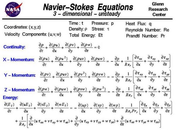
The Navier-Stokes equations consists of a time-dependent continuity equation for conservation of mass, three time-dependent conservation of momentum equations and a time-dependent conservation of energy equation. There are four independent variables in the problem, the x, y, and z spatial coordinates of some domain, and the time t. There are six dependent variables; the pressure p, density rho (\(\bf\rho\)), and temperature T (which is contained in the energy equation through the total energy Et) and three components of the velocity vector; the u component is in the x direction, the v component is in the y direction, and the w component is in the z direction. All of the dependent variables are functions of all four independent variables. The differential equations are therefore partial differential equations and not the ordinary differential equations that you study in a beginning calculus class. The partial derivative indicates that we are to hold all of the independent variables fixed, except the variable next to symbol, when computing a derivative. The set of equations are:

\(\Large \text{Continuity: }\frac{\partial p}{\partial t}+\frac{\partial (\rho u)}{\partial x}+\frac{\partial (\rho w)}{\partial z}=0\)

\(\Large \text{X-Momentum: }\frac{\partial(\rho u)}{\partial t}+\frac{\partial(\rho u^{2})}{\partial x}+\frac{\partial(\rho uv)}{\partial y}+\frac{\partial(\rho uw)}{\partial z}=\\\Large-\frac{\partial \rho}{\partial x}+\frac{1}{\mathit{Re}_{r}}[\frac{\partial \tau_{xx}}{\partial x}+\frac{\partial \tau_{xy}}{\partial y}+\frac{\partial \tau_{xz}}{\partial z}]\)

\(\Large \text{Y-Momentum: }\frac{\partial(\rho v)}{\partial t}+\frac{\partial(\rho uv)}{\partial x}+\frac{\partial(\rho v^{2})}{\partial y}+\frac{\partial(\rho uw)}{\partial z}=\\\Large-\frac{\partial \rho}{\partial y}+\frac{1}{\mathit{Re}_{r}}[\frac{\partial \tau_{xy}}{\partial x}+\frac{\partial \tau_{yy}}{\partial y}+\frac{\partial \tau_{yz}}{\partial z}]\)

\(\Large \text{Z-Momentum: }\frac{\partial(\rho w)}{\partial t}+\frac{\partial(\rho uw)}{\partial x}+\frac{\partial(\rho uw)}{\partial y}+\frac{\partial(\rho w^{2})}{\partial z}=\\\Large-\frac{\partial \rho}{\partial z}+\frac{1}{\mathit{Re}_{r}}[\frac{\partial \tau_{xz}}{\partial x}+\frac{\partial \tau_{yz}}{\partial y}+\frac{\partial \tau_{zz}}{\partial z}]\)

\(\Large \text{Energy: }\frac{\partial (E_{t})}{\partial t}+\frac{\partial (uE_{t})}{\partial x}+\frac{\partial (vE_{t})}{\partial y}+\frac{\partial (wE_{t})}{\partial z}=-\frac{\partial (up)}{\partial x}-\frac{\partial (vp)}{\partial y}-\\\Large\frac{\partial (wp)}{\partial z}-\frac{1}{\mathit{Re}_{r}\mathit{Pr}_{r}}[\frac{\partial q_{x}}{\partial x}+\frac{\partial q_{y}}{\partial y}+\frac{\partial q_{z}}{\partial z}]+\frac{1}{\mathit{Re}_{r}}[\frac{\partial}{\partial x}(u\tau_{xx}+v\tau_{xy}\\\Large+w\tau_{xz})+\frac{\partial}{\partial y}(u\tau_{xy}+v\tau_{yy}+w\tau_{yz})+\frac{\partial}{\partial z}(u\tau_{xz}+v\tau_{yz}+w\tau_{zz})]\)

where Re is the Reynolds number which is a similarity parameter that is the ratio of the scaling of the inertia of the flow to the viscous forces in the flow. The q variables are the heat flux components and Pr is the Prandtl number which is a similarity parameter that is the ratio of the viscous stresses to the thermal stresses. The tau (\(\bf \tau\)) variables are components of the stress tensor. A tensor is generated when you multiply two vectors in a certain way. Our velocity vector has three components; the stress tensor has nine components. Each component of the stress tensor is itself a second derivative of the velocity components.

Convection and Diffusion Terms

The terms on the left hand side of the momentum equations are called the convection terms of the equations. Convection is a physical process that occurs in a flow of gas in which some property is transported by the ordered motion of the flow. The terms on the right hand side of the momentum equations that are multiplied by the inverse Reynolds number are called the diffusion terms. Diffusion is a physical process that occurs in a flow of gas in which some property is transported by the random motion of the molecules of the gas. Diffusion is related to the stress tensor and to the viscosity of the gas. Turbulence, and the generation of boundary layers, are the result of diffusion in the flow. The Euler equations contain only the convection terms of the Navier-Stokes equations and can not, therefore, model boundary layers. There is a special simplification of the Navier-Stokes equations that describe boundary layer flows.

Note

Notice that all of the dependent variables appear in each equation. To solve a flow problem, you have to solve all five equations simultaneously. That is why we call this a coupled system of equations. There are actually some other equation that are required to solve this system. We only show five equations for six unknowns. An equation of state relates the pressure, temperature, and density of the gas. And we need to specify all of the terms of the stress tensor. In CFD the stress tensor terms are often approximated by a turbulence model.