Panel Code Performance Prediction

Engineers make mathematical predictions of the performance of any new aircraft as part of the design process. These predictions use the best data and mathematical techniques which are available to the engineer. For our full scale replica of the Wright 1900 aircraft, we have also made mathematical predictions of the aircraft performance. These computations were performed by Eric McFarland of NASA’s Glenn Research Center using a panel method which is normally used to compute the flow through turbine engine compressors. This program can compute the interaction of the top and bottom wings, the canard, and the ground.

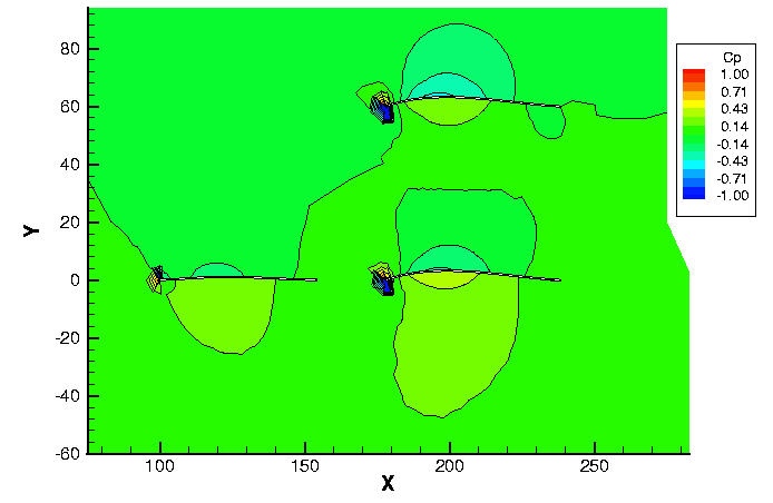
The figure at the top of this page shows the pressure distribution around the aircraft. The computation was performed for a wind velocity of fifteen miles per hour, and the aircraft flying five feet above the ground. The computed pressure is color coded and you can determine the value of the pressure by comparing to the color bar. With this computation, we see that most of the pressure changes take place near the leading edge of the airfoil. The pressure on the upper surface of each wing is lower than the pressure on the bottom surface. Notice that the pressure on the top wing is slightly different than the pressure on the bottom wing because the flow around each wing interacts with the other. We can look at the computed data in a slightly different way to better interpret the results of the calculation.

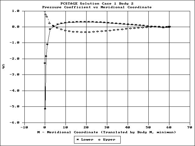
Here we have plotted the computed pressure around the lower wing. The “o”‘s are the pressure on the upper surface, the “x”‘s are the pressure on the lower surface. This plot uses the same data that was used for the contour plot; it is just presented differently. It’s much easier to see that the pressure on the lower surface is higher than the pressure on the upper surface. And using this graph we can determine the exact amount of the difference. Detailed data at zero, five, and ten degrees angle of attack are presented on separate pages. Using the information from these cases, we can develop plots of the aircraft performance versus angle of attack.

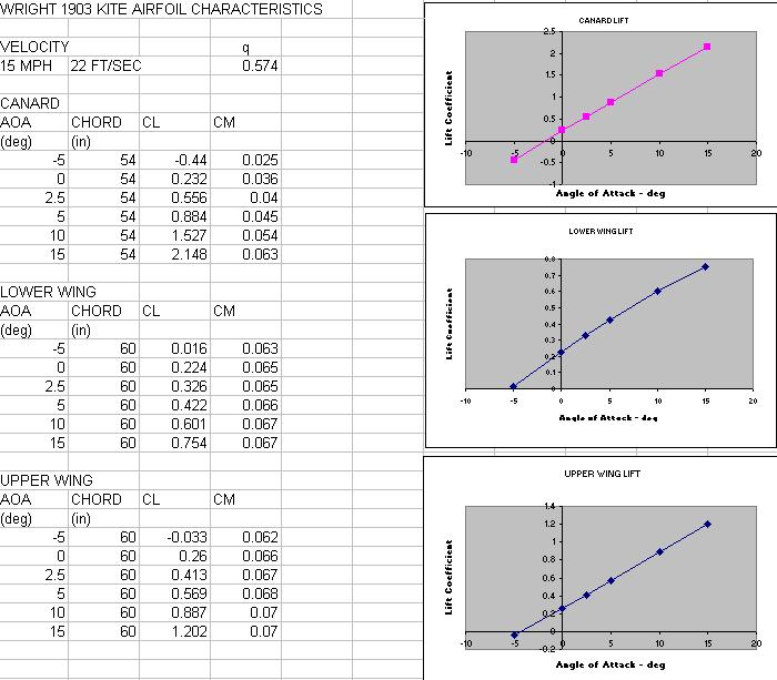
This analysis is performed for ideal flow conditions and can not predict the wing stall which may occur for higher angles of attack. However, we can use this data and the lift equation to determine the angle of attack necessary to lift the aircraft in a 15 mph wind. If we take the average lift coefficient (CL) of the top and bottom wing at 10 degrees angle of attack we get an aircraft CL = .74. The replica has a wing area (A) = 170 square feet. For the standard atmosphere the air density (r) is .00237 slug/cubic feet. This gives a lift (L) at 15 mph (V) and 10 degrees angle of attack of 68 pounds. [ L = CL * .5 * r * V^2 * A] Since our aircraft weighs 60 pounds, it should fly at 10 degrees and 15 mph. Compare this answer with the result from the simpler interactive analysis at the same conditions and you will find that the more detailed prediction gives about one half the lift of the simple analysis. A more detailed analysis usually gives a more pessimistic answer because a simple analysis usually neglects effects which can be important.

We can take the computed results and produce an animation of the change in flight conditions. Notice in the animation the large blue region (very low pressure) which develops on the upper wing and canard at 10 degrees angle of attack (the largest positive value). This rather strong pressure variation may cause the air flow to separate at these conditions.